The most basic way to identify a team style of play is to look at possession percentages, pass success rates, tackle rates, the average number of faults per game, etc…. More recently a lot of work has been done with expected goal models which are pretty good to capture the quality of chances created and conceded. However, it only exposes a metric to the analytic audience and not a concrete vision of how a team plays. It’s still difficult to get knowledge of passes sequences types preferred for a given team during open plays.

The question of how to describe and analyse pass sequences is not new in the football analytics community. Works like those of David Permodo Meza in his “Passing Motifs: Identifying Team and Player Passing Style” post on Statsbomb  or “Visualizing passing sequences” by Ricardo Tavarez for Football Crunching  are worth reading and are kind of state of the art for analysing pass sequences in soccer.

In this blog post, we will explore a method based on deep learning to find some Premier League club possession patterns and trying to show how teams are quite different from each other.

I can’t start this piece without referring the work of Joe Mulberry, Director of Recruitment at Right2Dream (a company with a part of the Danish club FC Nordsjælland), and the great presentation  he gave during 2019 Opta Forum in London. The following analysis is strongly inspired by this one.

Encoding possession: a Possession2Vec model

Firstly, what is a possession? To keep it simple: it’s a flow of passes and moves until the team having the ball lose it. So it ends after an off-target shot, a success tackle from the opponent team, or an unsuccessful pass: when the other team is gaining the possession of the ball.

Thanks to on-ball events, we can create a simple representation of these possessions by purely drawing white lines for passes. Here are some samples:

These images are 105 pixels wide and 68 pixels high, following average football field dimension. The direction of the attack is from left to right.

You will note that the time dimension is taken into account, with darker lines for the beginning of the action, the last pass being in pure white. Spaces between the lines are player runs which we can’t draw here because tracking data are still rare.

Building these images for the last three seasons of Premier League we can work with a decent dataset. Each image can be flattened in 105x68=7140 dimensions vectors.

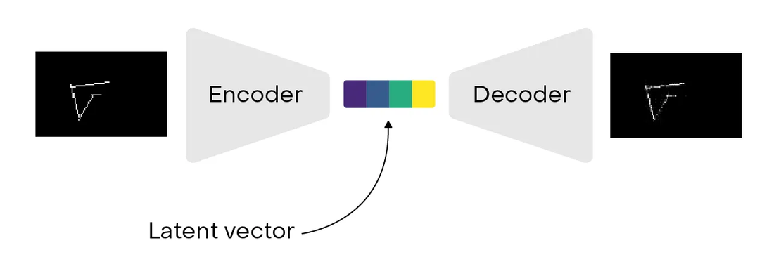
To be able to compare these vectors, we use what is known as an auto-encoder in the deep learning field. Auto-encoders are specific types of neural networks architecture which allow to encode an input into a compressed representation and then get back to almost original data with a decoding function.

By design, these compressed representations — also known as latent vectors — are pretty useful to reduce input dimension but also to keep similarity between data. In my experiments, I chose to set dimensions of these vectors to 256. Choosing a very low dimension here would ask more training time and will probably make things harder to keep original data information.

Moreover, to be able to visualize these informations, we can use a technique to further reduce the dimension of these latent vectors. We have high dimension and non-linear data so the t-SNE algorithm seems to be best suited for the operation.

Here is a view of all pass possessions represented over two dimension thanks to auto-encoder embeddings and so t-SNE algorithm.

Thankfully, after reducing images composed of 7140 pixels to only two dimensions, we are still able to keep information similarity between possessions. You might note this graphic highlight number of passes by possession and we see how data are already a bit clustered.

To be able to compare teams possessions, we bucketize these data points with K-means algorithm. The number of clusters is chosen arbitrarily while using a technique such as the Elbow method is not particularly needed: more the number is higher more we have detailed clusters. We will first look at results with 25 buckets and then going deeper with 500 buckets.

Note that we could also simply group this data by framing them, but K-means allows to be a little more precise.

A general look at large scale results

By simply looking at team distribution in each cluster, we can find out what are the preferences of the teams or what kind of possession they use the most compared to others.

We filter teams to get rid of ones where we have less data, those which have been relegated or promoted over the last three seasons: Brighton, Fulham, Huddersfield, Sunderland, Wolverhampton, Middlesbrough, Norwich, Aston Villa, Cardiff, Newcastle.

Heatmap above shows team distribution in each cluster (k=25). Among interesting insights, we can see how Manchester City is quite different from other teams. Looking at some samples of possession in cluster n°4 highlight Manchester City style of play, with long possession in a high position.

Without surprise, other teams well placed in cluster n°4 are Arsenal, Tottenham, Liverpool or Chelsea. Conversely, cluster n°3 highlights teams playing long balls such as Leicester or Swansea

Looking at some specific cluster, for instance cluster n°14 is also interesting.

Manchester City, Arsenal and Tottenham are pretty bad in it. Looking at some samples and we see that this cluster represent short possessions on right sides, from right backs to midfielders. Fact that these three teams have regular difficulties to build up from this wing show the power of this modelisation which can capture such informations.

Going into the details

If we look at data clustered in 500 buckets we can appreciate much more details in possessions types. By looking for big differences in cluster distribution we can find team specificities

West Ham is almost alone on cluster n°17 which represent very short pass on the right wing. With a lot of games lining five defenders among Zabaleta and Antonio the right side, Hammers are strong on this side of the pitch.

Looking at where a team as a low proportion of actions is also interesting. For example, Leicester has the lowest distribution in cluster n°53. This one corresponds to built phases from the centre to the left side of the fields.

Over the last 3 seasons, players in these areas are Fuchs or Albrighton who are not the best players of Leicester for build-up. Moreover, this didn’t change recently with either Madison or Gray which are two great players but not likely to go so deeper in their part.

At the opposite, Foxes are present in cluster n°455 which is equal to sequence on the right side with “inside” passes. Is it Mahrez influence? Difficult to say but the fact the second team in this bucket is Tottenham with Eriksen playing a specific role on this side (difficult to find a player to compare with him in the league, he’s kind of unique).

We can try another exercise: taking Arsenal as an example, where the Gunners are the most different from other teams and so how to concentrate when defending against them?

Arsenal are almost alone in n° 361 and n° 287:

While the first one is quite surprising the second one is probably representative of a trained tactic with action beginning on the left side and quickly changing to the right side with a long ball ending with a chance to an open cross. Without surprise, the second team in cluster n°287 is Manchester City. Opposite teams would like to pay attention on this side when defending against these teams.

Possible improvements

This framework is quite good to capture pass sequences style and to see where and how teams prefer to play. However, there are still ways of improvements:

• While we concentrate on teams, we could also take a deeper a look at player levels, and so compare players by differencing them on how they are involved in passes sequences.
• By changing coordinate referential, we’ll probably appreciate patterns of pass sequences whatever their pitch position. So we will probably see specific combinations worked during training or some players palatability.
• Something really basic is to predict game results thanks to team statistics (average possession, xG per game, position in the leaderboard, bookmaker odds, etc…). I tried to take only these latent vectors as features to characterize teams: we can predict games results with 50% accuracy with a simple logistic regression, which is pretty good with so few features.

Resources

Here are some resources which help me a lot to write this blog post:

• Joe Mulberry  presentation during 2019 Opta Forum  in London.
• “Experiments on Clustering Possession Sequences”  from Garry Gelade .
• “Finding Interesting Pass Patterns from Soccer Game Records”  from Shoji Hirano and Shusaku Tsumoto (Department of Medical Informatics, Shimane University, School of Medicine, Japan).
• “A metallurgical scientist’s approach to predicting NBA team success”  by Peter Tsai.
• “Building Autoencoders in Keras”  by François Chollet  on The Keras Blog.