Or how to 3D print (almost) any places in the world.

If you’re listening to the R community, you may have heard about the rayshader package recently released by the formidable Tyler Morgan-Wall , Ph.D. in Physics from Johns Hopkins University, and a BA in Physics from the University of Pennsylvania.

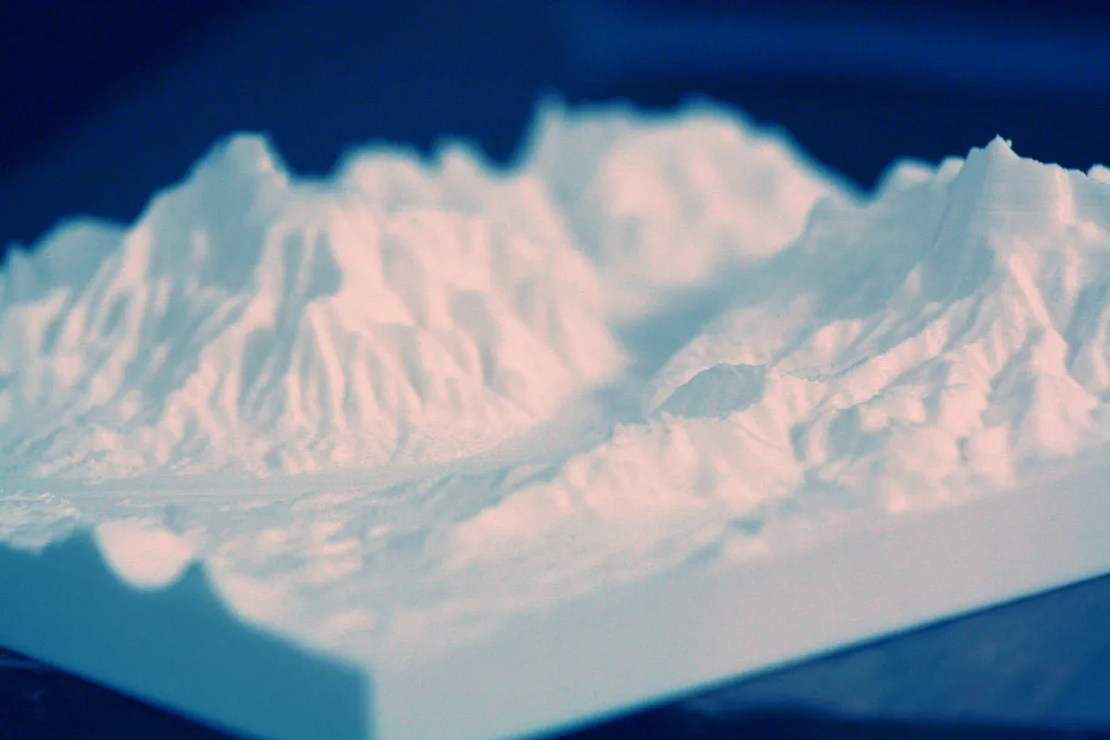
Rayshader is a mapping-package for producing and visualizing hillshaded maps from elevation matrices, in 2D and 3D. With this library, we can plot and print any places in the world with pretty fine details of the topography.

Following paragraphs show how you can run this piece of software on your computer, where you can find elevation data for almost any place in the world and how to plot and 3D print those places.

Note that is more a personal note of rayshader package than a full review. For full explanations of all features, you can check the repository on GitHub directly: https://github.com/tylermorganwall/rayshader

Workspace and installation

As I used to work essentially within a Docker environment, I build a Dockerfile based on the awesome rocker project (https://www.rocker-project.org/ ) with all dependencies pre-installed, so you can run the following commands to get a Rstudio environment (exposing Rstudio to your web browser) with rayshader installed and your data mapped into the container:

git clone <https://gitlab.com/ben8t/rayshader_experiment.git>  
cd rayshader_experiment  
docker build -t rayshader .  
docker container run -d --rm -v $(pwd):/home/rstudio/kitematic -p 8787:8787 -e USER=admin -e PASSWORD=root --name rstudio rayshader

However, if don’t know about Docker, you can find all explanations from Michael Galarnyk  pieces to install R on your computer (macOS, Linux or Windows):

https://medium.com/@GalarnykMichael/install-r-and-rstudio-on-ubuntu-12-04-14-04-16-04-b6b3107f7779

https://medium.com/@GalarnykMichael/install-r-and-rstudio-on-mac-e911606ce4f4

https://medium.com/@GalarnykMichael/install-r-and-rstudio-on-windows-5f503f708027

Then you can install without too many difficulties the last release of rayshader package with the following commands:

library(devtools)  
install_github('tylermorganwall/rayshader')

Where do we find elevation data?

There are in fact a lot different sources of elevation data.

In developed countries, there are a lot of “open data” platforms where you can find whatever data you want, and sometimes elevation data.

NASA, with the Space Shuttle Radar Topography Mission, captured Earth’s topography at 1 arc-second (30 meters) for over 80% of the Earth’s surface.

https://gisgeography.com/srtm-shuttle-radar-topography-mission

You will find an online explorer with a lot of dataset in the following article:

https://gisgeography.com/usgs-earth-explorer-download-free-landsat-imagery

Here are some other links where you’ll find resources:

https://gisgeography.com/free-global-dem-data-sources

http://opendata.apur.org/datasets/hauteur-bati-2012  (France data)

https://openmaptiles.com

https://www.lib.ncsu.edu/gis/elevation

(just type “elevation data <place you want>” in your search engine and you’ll find a lot of sources too).

It will probably need to be done on a case by case basis to find the perfect data, but the fact is that it is quite easy to find a reliable source.

Plotting in 2D or 3D

The rayshader package comes with some demo. Therefore you can run the following command to take a look at some expected results:

library(rayshader)  
montereybay %>%  
    sphere_shade(texture="imhof2") %>%  
    plot_map()montereybay %>%  
    sphere_shade(texture="imhof2") %>%  
    plot_3d(montereybay, zscale=50)

Note that if you are into a Docker container you might see the graph view while it lacks some display utilities. You can “solve” this problem by saving the 3D shape to a STL file (code in the last part) and using an online viewer like https://www.viewstl.com/ . If you are on a local installation you will not have that kind of problem.

Using your data

In this example, I’m using a small sample of Paris building elevation data. However, you can use whatever place you will find.

raster::raster("local_data.tif") -> localtif  
elmat = matrix(raster::extract(localtif,raster::extent(localtif),buffer=1000),  
               nrow=ncol(localtif),ncol=nrow(localtif))elmat %>%  
    sphere_shade(texture = "imhof3") %>%  
    add_shadow(ray_shade(elmat,lambert = TRUE),0.7) %>%  
    plot_map(rotate=0)

For 3d plot:

raster::raster("local_data.tif") -> localtif  
elmat = matrix(raster::extract(localtif,raster::extent(localtif),buffer=1000),  
               nrow=ncol(localtif),ncol=nrow(localtif))elmat %>%  
    sphere_shade(texture = "unicorn") %>%  
    add_shadow(ray_shade(elmat,lambert = TRUE),0.2) %>%  
    plot_3d(elmat)

3D printing

Using save_3dprint() rayshader feature, we can save this 3D rendering to a STL file:

raster::raster("local_data.tif") -> localtif  
elmat = matrix(raster::extract(localtif,raster::extent(localtif),buffer=1000),  
               nrow=ncol(localtif),ncol=nrow(localtif))elmat %>%  
    sphere_shade(texture = "unicorn") %>%  
    add_shadow(ray_shade(elmat,lambert = TRUE),0.2) %>%  
    plot_3d(elmat, baseshape="circle")  
save_3dprint("local_data.stl")

Then if you a 3D print at home you can deal with this file, but like almost everybody, we’ll have to send this file to a professional service which 3D print the file for us.

You can take a look at 3Dhubs (https://www.3dhubs.com/ ) which offers his services for a fairly reasonable cost. Here is an example from Tyler Tran on Philadelphia data.

3D printed my neighborhood using @tylermorganwall ‘s rayshader and data from @opendataphilly ! pic.twitter.com/PO5pYFckjB

— Tyler Tran (@tylerjtran) January 9, 2019

Conclusion

Thanks to the rayshader package, we can plot and print in 3D any elevation data we can find. With all that lidar data coming from the self-driving car industry, there is a lot of experiments we can do.

Again, thanks to Tyler Morgan-Wall who release this formidable library. Go take a look at his blog  or follow him on Twitter . It’s worthwhile.

Hope you like the reading, don’t hesitate to test these commands and leave a response below.